So, You Want To Write a Raytracer?

Introduction

I have written quite a large amount about writing diffraction propagation and other physical optics software. I had some down time during an explosive COVID wave this winter, and decided I would spend some of it writing a ray tracer.

A major weakness of diffraction modeling is that it cannot account for what really happens when optics are misaligned, and is usually pre-fed by linear sensitivity matricies which have unknown domains of validity and leave out the fun of things like changes in pupil aberrations. It seems natural that the highest fidelity of modeling is a hybrid approach which utilizes raytracing to figure out what really happened, then uses wave propagation to accurately capture it.

Before anyone gets too excited, I’m not out to eat optical design software’s lunch. This is intended to be an analysis tool. It’s actually fairly zippy for something with a core banged out in a 1 FTE x 1 day or so. It’s not actually very slow – 2.5 million ray-surfaces per second on a laptop CPU, with full GPU compatability for > 1000x faster speeds at scale. Not bad for pure python.

I have long found two resources to be seminal on ray-tracing: the Finite Raytracing chapters in Welford’s Aberrations of Optical Systems, and Spencer & Murty’s 1961 JOSA paper, General Ray-Trace Procedure. The Spencer & Murty paper has a more modern or approachable syntax, despite being 20 years older. And it labors less over “special” types of surfaces, which dominate the pages of Welford’s chapters. Just be mindful of Horwitz’ 1991 correction for the fourth step. This post will be something of a tutorial on implementing their paper, so turn away now or break out your highlighters and notebooks. I’ll also suggest the source code of Mike Hayford’s ray-optics and Gavin Niendorf’s TracePy, if you want to look over things written by folks whose brains work a bit different to mine.

Before going further, a ray is described by its position and direction cosines. The latter essentially describe the direction in which it will travel in the future, or the “orientation” of the ray. $$\begin{array}{rl}P& =⟨X,Y,Z⟩\\ S& =⟨k,l,m⟩\end{array}$$ The S&M paper describes raytracing as four basic steps:

1. (optional) Translate and rotate the ray from a global coordinate system to the surface’s local coordinate system
2. Intersect the ray with the surface
3. Reflect or refract the ray
4. (optional) return to the global coordinate system

Global to Local Coordinates

To perform the first step is easy, $$\begin{array}{rl}R& =\left[\begin{array}{ccc}{R}_{00}& R_{01}& R_{02}\\ R_{10}& R_{11}& R_{12}\\ R_{20}& R_{21}& R_{22}\end{array}\right]\\ P^{\prime }& =R\left[\begin{array}{c}X-X_0\\ Y-Y_0\\ Z-Z_0\end{array}\right]\\ S^{\prime }& =R\left[\begin{array}{c}k\\ l\\ m\end{array}\right]\end{array}$$ where $R$ is a 3x3 rotation matrix, and the column vectors are $P$ and some origin point for the local coordinate system, $O$. Simply subtract $O$ from $P$, then do the matrix-vector product with R. It’s all one line of code. And S is just the matrix-vector product. To build R, simply type in wikipedia. There’s not much to say here, and this step is optional.

Ray-Surface intersection

Ray intersection relies on some special tricks S&M have come up with. First, their peculiar definition of an optical surface, $$F(X,Y,Z)=0$$ is not just some weird 1960s syntax. They really do mean this to be zero, and as it turns out what it really means is $$F(X,Y,Z)=Z-G(X,Y)$$ where $G$ is the surface sag function, say that of a sphere, or a conic, or Q2D polynomials with a base off-axis conic. Ray-surface intersection begins by advancing the ray to where it reaches $Z=0$, which is done by computing $-Z/m$, multiplying $S$ by that scalar, and adding it to the current $P$: $$P_0=P+(-Z/m)S$$ Going here first simplifies S&M’s algebra that follows. They basically want to find the root of an equation (remember, F=0). Starting from zero guarantees that by moving in a particular direction, the correct (real, non-imaginary) root is chosen. From here, iteration is done, since ray-surface intersection is not closed form in general. To find the distance $s$ along the ray which results in intersection between the ray and surface, S&M use Newton’s method, which requires you to be able to compute the sag of the surface, and its normal vector $r=⟨N_x,N_y,N_z⟩=\mathrm{\nabla }F$ for any point $P$. The normal vector is simply the negative of the partial derivatives of the sag (the negative sign in front of $G$ in the previous equation) with respect to X and Y, and 1.0 in the Z direction, gven the leading $Z$ term in our expression for F.

Computing these derivatives is laborious for more complex surface geometries. S&M give an answer for conics, but their definition of a conic is different to the colloquial one, so I don’t suggest using theirs. The chain and product rule, done by hand, are how I did it for every polynomial in prysm you’d care about (including Zernikes and all three kinds of Q polynomial).

Given those two capabilities, begin from $s_0=0$, and iterate with: $$s_{n+1}=s_n-F/(r\cdot S)$$ when $|s_{n+1}-s|$ is less then some tolerance, or an iteration limit has been reached, the algorithm concludes. $r\cdot S$ is the dot product between $r$ and $S$. For a parabola, this will converge in one iteration since the derivative is linear. Neat!

At the end of these iterations, the point which intersects the surface is $$P_i=P_0+s_{n}S$$

Reflection and Refraction

Reflection is simple, $$S^{\prime }=S-2\circ \frac{S\cdot r}{N_x^2+N_y^2+N_z^2}\circ r$$ In this equation, $\circ$ is the Hadamard (elementwise) product and $\cdot$ the dot product. The large radical expression in the middle is the direction cosine between the surface normal and incident ray.

No iteration is required, and the surface intersection function will give us the final value of $r$ as an ending product. As well, $S$ has not changed at all, so we already have that.

S&M solve refraction by using iteration. It’s not immediately obvious to me why they chose to do that, since it’s fairly expensive to do so. Instead here I’ll just show the final answer after working through the vectorial form of Snell’s law to the final answer, $$\begin{array}{rl}\mu & =n/n^{\prime }\\ r^{\prime }& =\sqrt{1-{\mu }^2[1-(S\cdot r{)}^2]}\circ r+\mu [S-(S\cdot r)\circ r]\end{array}$$ This is a bit of a bear of an expression, but it’s very compact when written out with numpy, and the same dot product is in it twice.

The final step contains an error in S&M (Horwitz 1991) and should be written as the first step in reverse, $$\begin{array}{rl}{P}^{\prime }& =\left(R^T\left[\begin{array}{c}X\\ Y\\ Z\end{array}\right]\right)+O\\ S^{\prime }& =R^T\left[\begin{array}{c}k\\ l\\ m\end{array}\right]\end{array}$$

With those things done, you have completed an implementation of a raytracer. And, like me, you will find it takes about 50 microseconds per ray-surface – 20,000 ray-surfaces per second. But didn’t I say 2.5 million?

Performance

The fantastic thing about numpy is that it allows you to write code that very clearly implements numerical algorithms that operate on arrays. And, if those arrays are big enough, it’s at least as fast as a totally expert numerics programmer in C++ or Fortran. After all, a hundred of those people have been optimizing Numpy for 20 years. Just try to using Eigen or hand rolled code, You will be amazed how hard it is to even hit par. Or, like me you can write an experiment in a better compiled language than C++, and find that you can do twice as fast as numpy in exchange for having no access to plotting libraries or an easy way to call the code from an environment anyone wants to use it from. Twice as fast is still 500x slower than the GPU using Cupy, which requires no source code changes to the python. So you can imagine which I’m more interested in.

Anyway. If you have to do many tiny calculations – and the 3 element vectors here are tiny – you can actually batch them with numpy, paying the python tax only once for all of them. For example, if you want to do the matrix-vector product between $R$ and $P$, numpy pretends $P$ is 1x3 and does a matmul. If you made $R$ be shape (N,3,3) instead and P were (N,3,1), numpy would do all the matrix products at once. The result for moderate to large N is about a 100x speedup, the speed gap between a Python loop and a C loop. For all of our dot products, there is no BLAS way to do it, which is a shame. My least favorite tensor algebra tool, einsum, comes to the rescue with a solution that’s about 50% slower than a mysterious testing function numpy doesn’t want you using. Anyway, to batch dot products just do np.einsum('ij,ij->i', S, R). The syntax is cryptic.

Inside the intersection, you simply need to keep a mask around of which rays have/have not converged and only iterate those rays which have not converged. This is implemented in the source code of prysm. I won’t explain it here, since it’t just bookkeeping. This is the biggest tax paid, since for the first time it invents work done purely for the parallel processing, which wouldn’t exist in a simple for loop in a compiled language.

The API is the same for batch raytraces and for single raytraces, simply give P and S to the raytrace function with a prescription. If P has one dimension it’s a scalar ray trace, and if it has two it’s a batch raytrace. Internally a scalar raytrace is expanded to an N=1 batch raytrace so the code can be the same.

I did a deep dive I wont’ blabber about here, and found that even with multithreading I can only go 2-3x faster than the python code single threaded by parallelizing it, which wasn’t very complicated. So to scale to lots of cores, boy oh boy do you need lots of memory bandwidth (hello, DDR5?) At least the Nvidia A100 has checks notes 2TB/s of memory bandwidth, 40x that of my laptop.

Creature Comforts

No raytrace is any good without the ability to make ray fans or grids, aim rays, draw raytrace plots, or do basic solves like for the paraxial image location.

A PIM solve can be implemented by tracing rays near the paraxial regime along the x=0 or y=0 spines and finding where they intersect each other. This is robust in ways that tallying up element powers and object locations is not. Simply trace one pair of rays in Y and one in X and intersect the two pairs. The average of those two locations is the paraxial image location.

Matplotlib is happy to draw line groups by giving it column vectors, so we just unpack the final axis of the history of $P$, and plotting ax.plot(phist[..., 2], phist[..., 1]) for a Z-Y plot. It’s even pretty fast (1.3 sec for 4096 rays, 25 ms for 32 rays). Generating ray grids is just a little front-end API to making 1D arrays of X,Y,Z and stacking them with mirrored direction cosines (which begin as $⟨0,0,1⟩$ and just need a multiply with $R$ to make X and Y field angles). Drawing the optical surfaces, at least for reflective systems, is just evaluating the sag function and plotting a black line. Well, sort of. I haven’t figured out how to draw tilted surfaces ($R\ne \text{None}$) yet.

All and all, this is about a thousand lines of code for a ray tracer with asymptotic performance similar to the state of the art, with most of the needed creature comforts. Supporting new surface geometries is less than ten lines of code each by using the rich polynomials module of prysm and its coordinate centric design (as opposed to npix).

All in all, pretty nice.

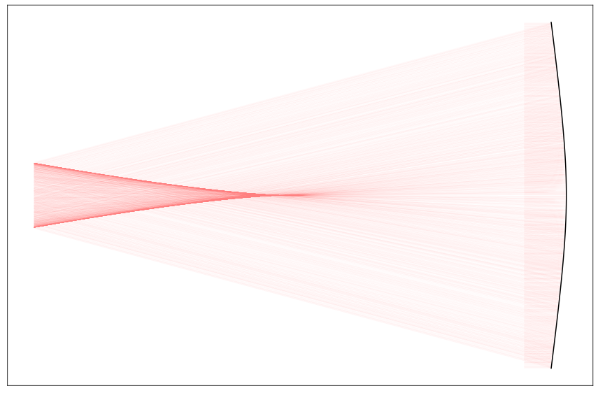
I’ll close this with a piece of art, made by tracing a few thousand rays and plotting them with some transparency to show the caustics. It’s simply a concave mirror with a very large conic constant (-50). The caustic makes the appearance of Cassegrain family telescope with only one mirror.