Phase Retrieval VI: Faster Nonlinear Optimization, Deeper Insight

In the last post, I showed the efficacy of nonlinear optimization for phase retrieval. In it, I mentioned the algorithm used to do the optimization itself would like to know the gradient of the cost function with respect to the parameters, and if not given the optimization package usually uses finite differences to get the gradient on its own. Since we do not, in general, know the analytic PSF associated with a given phase error, or even a more general amplitude function this may seem like an intractable task, but it is not so. We can use a process known as automatic differentiation to compute the gradients. A full tutorial on this is outside the scope of this post - see Alden Jurling’s publications on the topic for more detail. In this post, I’ll use similar notation as Jurling2014 in JOSA A (which is very similar to Fienup1982).

Basics of Algorithmic Differentiation

If we have the pupil function:

$$ g = A \exp(i\frac{2\pi}{\lambda}\Theta(g)) $$

This looks cyclic, so we’ll replace $\Theta(g)$ with $\mathbf{W}$, the same variable Alden used:

$$ g = A \exp(i\frac{2\pi}{\lambda}\mathbf{W}) $$

The field in the focal plane is

$$ G = \mathfrak{F}[g] $$

with the slightly more general notation FT, vs FFT. The intensity

$$ I = |G|^2 $$

Our error metric is:

$$ \sum [I - D]^2 $$

for data $D$ (measurements, $|F|^2$).

Following Alden’s 2014 scriptures, we can write a forward and backward (adjoint) model in two columns: $$ \begin{align} & \text{(optional)} & \partial_aE &= \overline{\mathbf{W}} \cdot Z_j \\
\mathbf{W} &= \sum_n a_n Z_n & \overline{\mathbf{W}} &= \frac{2\pi}{\lambda} \Im[\overline{g}] \\
g &= A \exp{i\frac{2\pi}{\lambda} \mathbf{W}} & \overline{g} &= \mathfrak{F}^{-1}[\overline{G}] \\
G &= \mathfrak{F}[g] & \overline{G} &= 2(G \cdot I) \\
I &= |G|^2 & \overline{I} &= 2 (I-D) \\
E &= \sum [I-D]^2 \\
\end{align} $$

(read left top to bottom, right bottom to top)

The top step in the reverse pass is optional, and projects the elementwise gradient $\overline{\mathbf{W}}$ into some basis set $Z_j$. $a_j$ are the coefficients, and $\overline{\mathbf{W}} \cdot Z_j$ is a tensor product between the 3D array $Z_j$ and 2D array $\overline{\mathbf{W}}$, resulting in a vector of length $j$.

This procedure allows us to substitute the update step from the second post inside the conjugate gradient method with any optimization procedure we like, so long as we provide either $\overline{\mathbf{W}}$ or $\partial_aE$.

In terms of an efficient implementation, notice that several variables formed or updated on the forward pass (left column) are re-used on the reverse pass (right column). It is best to wrap this computation in some container for the state (a class, a dictionary, etc). For example:

def ft_fwd(x):
    return fft.fft2(x, norm='ortho')

def ft_rev(x):
    return fft.ifft2(x, norm='ortho')

class NLOptPRModel:
    def __init__(self, amp, wvl, basis, data):
        self.amp = amp
        self.wvl = wvl
        self.basis = basis
        self.D = data
        self.hist = []

    def logcallback(self, x):
        self.hist.append(x.copy())

    def update(self, x):
        phs = np.tensordot(basis, x, axes=(0,0))
        W = (2 * np.pi / self.wvl) * phs
        g = self.amp * np.exp(1j * W)
        G = ft_fwd(g)
        I = np.abs(G)**2
        E = np.sum((I-self.D)**2)
        self.W = W
        self.g = g
        self.G = G
        self.I = I
        self.E = E
        return

    def fwd(self, x):
        self.update(x)
        return self.E

    def rev(self, x):
        self.update(x)
        Ibar = 2 * (self.I - self.D)
        Gbar = 2 * Ibar * self.G
        gbar = ft_rev(Gbar)
        Wbar = 2 * np.pi / self.wvl * np.imag(gbar * np.conj(self.g))
        abar = np.tensordot(self.basis, Wbar)
        self.Ibar = Ibar
        self.Gbar = Gbar
        self.gbar = gbar
        self.Wbar = Wbar
        self.abar = abar
        return self.abar

The ft_fwd and ft_rev functions can include shifts at your preference. norm='ortho' makes them satisfy Parseval’s theorem, otherwise we would need to write gbar = ft_rev(Gbar) * Gbar.size with the typical FFT normalization rules.

Let’s see how this compares to finite differences. I’ll skip the data synthesis part, since it has been shown before. The optimizer will solve for Noll Z4..Z11, which is a low dimensional problem where finite differences is completely viable. As an aside, with real data you would need Z2,Z3 in the parameter space, or convergence will never happen, due to finite centering accuracy of the data. Anyway:

nlp = NLOptPRModel(amp, wvl, basis, data)
start = time.perf_counter()
res = optimize.minimize(nlp.fwd, coefs-(np.random.rand(len(coefs))*10), jac=nlp.rev, method='L-BFGS-B', options={'maxls': 20, 'ftol': 1e-17, 'gtol': 1e-17, 'maxiter': 200, 'disp': 1}, callback=nlp.logcallback)
end = time.perf_counter()
print('OPTIMIZATION TOOK', end-start)
print(res)

This takes 2.1 seconds. A second call, identical less the jac=, takes 7.3 seconds. Both of these are fast (in the same ballpark as pressing measure on a Fizeau interferometer, for example), but ~3.5x faster for 7 dimensions is roughly a speedup of $N/2$, which would become 18x faster for 36 modes, and more than 100,000 times faster for an elementwise solution.

Speaking of elementwise solutions, it is trivial to turn this modal solver into a zonal solver:

      # ... snip
      def update(self, x):
        phs = x.reshape(self.amp.shape)

      # no abar in rev, return self.Wbar.ravel()

This will run much slower and use a lot of memory, but can do about 200 iterations in about 12 seconds. Adding three lines of numpy slicing to remove all of the variables that control phase outside the pupil reduces the problem from dimension 262,000 to dimension 51,000 and speeds it up to 200 iterations in 7.4 seconds. That’s handy, because we like to use zonal solvers to touch up modal solutions with any elementwise content that does not project into their basis. That work flow simply looks like performing a modal solution, and passing nlp.phs from the modal answer as the x0 for the zonal optimization.

Diversity and Differentiation Together

The astute reader will notice a regression. In the last post, I showed how the modal solver could be fooled easily by the twin image problem, and we could very trivially add diversity to break the ambiguity. In the last section of this post, we have no diversity again, and so the ambiguity has returned. To add diversity, the adjoint model (nlp.rev) must be back-propagated for each diversity, and at the end the final gradient term $\overline{\mathbf{W}}$ or $\overline{a}$ (weighted) summed over the diversity index. If you are interested in the code for personal use, feel free to reach out but I won’t be posting it here.

What is more interesting is what can be learned from the intermediate data produced. For example, Bruce Dean has an excellent paper on focus diversity selection for phase retrieval. We can take a similar look, using only data produced by our phase retrieval problem. By plotting $\overline{\mathbf{W}}$ for each diversity, we can see what information lies in the defocus planes vs in the in-focus plane:

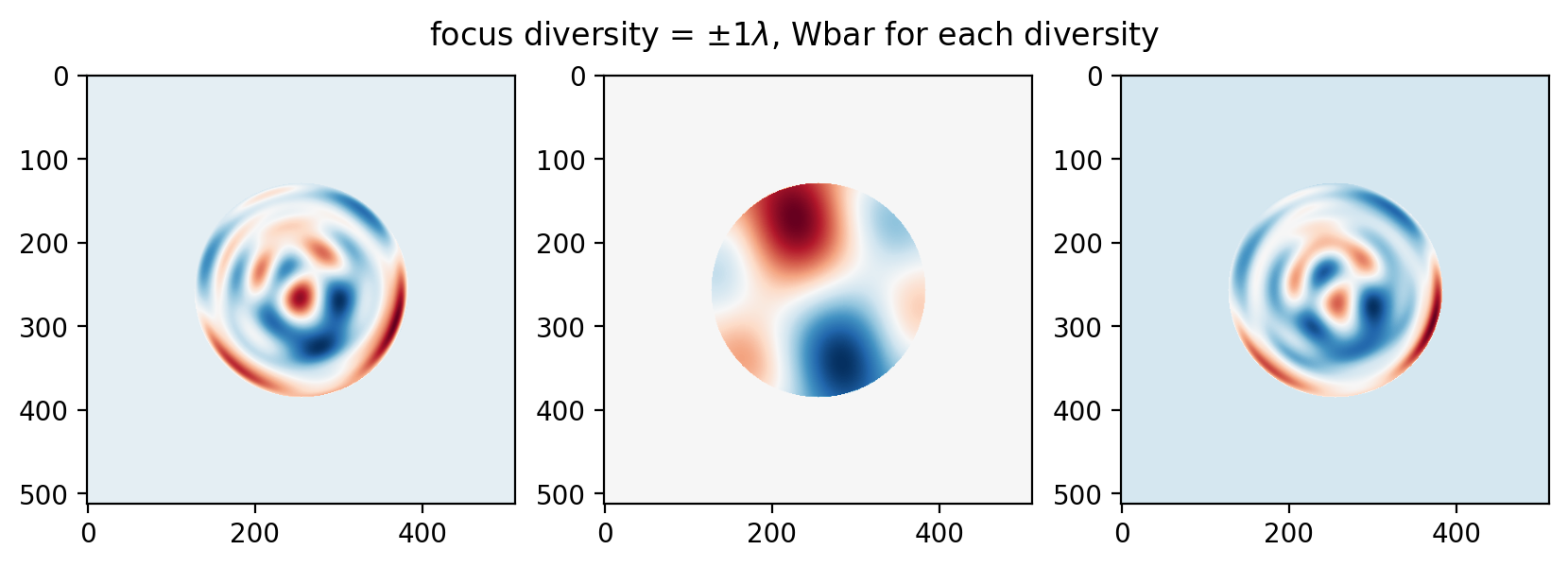
Some ripples are similar between the planes at 1 wave, at 3 waves the frequency of the ripples increases:

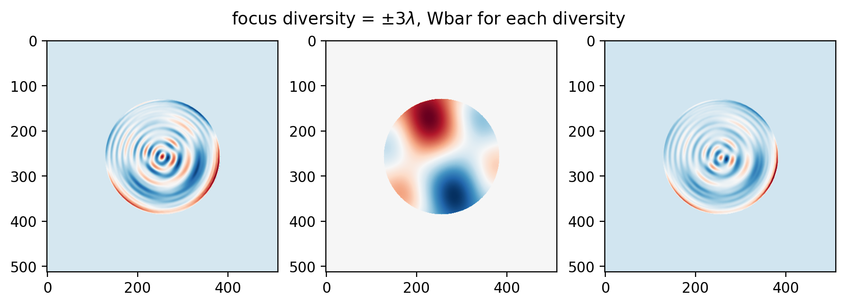
… and this trend continues to 5 waves (and beyond):

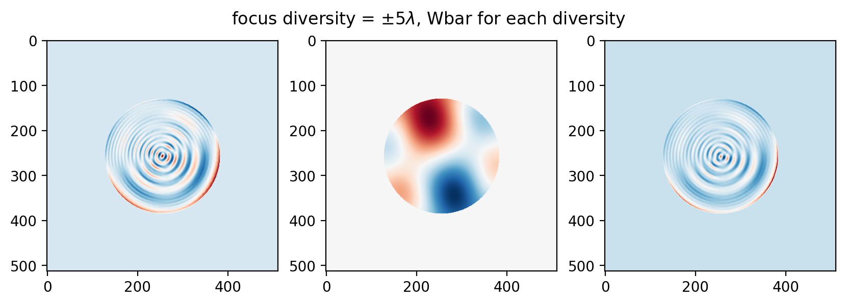
This is consistent with the final thrust of Bruce’s paper, that for higher frequency errors a larger diversity is desirable while for lower frequency errors a smaller diversity is desirable.

Wrap-up

This post has given an extremely brief tour of algorithmic differentiation, and its immense utility for image-based wavefront sensing. The benefits can be succinctly summarized in order of consequence as:

• algorithmic differentiation permits the use of state of the art optimizers for elementwise or “zonal” phase retrieval, with or without diversity. These algorithms substantially outperform contemporary iterative transform methods like Gerchberg-Saxton.

• algorithmic differentiation produces many intermediate data products, which are useful for the implementer or driver of the phase retrieval algorithm to study the physics, or diagnose the progress of the algorithm.

• algorithmic differentiation accelerates computation for phase retrieval, bringing it into a real-time performance class.

I may write one or two more posts at a higher level on how to use all of these things together (please make your voice heard if you are chomping at the bit for that), but this is about the end of our journey. We have covered up to and including the very state of the art in the field. There are no rabbits left in the hat.