Phase Retrieval IV: Diversity Basics

Last updated on Jan 16, 2023

Introduction

In the last post I showed the superiority of the Conjugate Gradient approach to phase retrieval over Gerchberg-Saxton, finding solutions that are at least an order of magnitude superior to GS. In the closing words, I alluded that as the phase error grew, the superiority of CG over GS would, too, improve.

The sample problem was carefully chosen to be one for which Phase Retrieval always works well; a phase error dominated (indeed, entirely made up of) low order features. In this post, we will examine what happens when the phase error contains substantial high frequency components, and the most common solution to that problem (focus diversity).

At the outset, we will repeat the same exact forward and reverse model as last time, but change one early parameter:

nms = [polynomials.noll_to_nm(j) for j in range(3,160)]
coefs = np.random.rand(len(nms)) * 1  # nm rms

That is, we will use about 10x as many Zernike modes, which includes many higher frequency components. Running GS and CG for 500 iterations produces the following convergence:

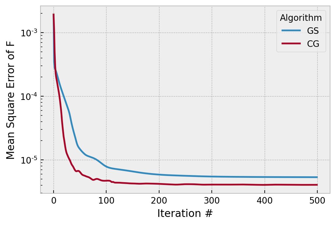
cost vs iteration for GS and CG PR algorithms

In this case, GS does better (the phase is a better match), but CG appears to do better (CG finds superior data consistency). What has happened here is that the high frequency phase components are ambiguous in a single PSF, so neither CG nor GS can find a particularly great solution, and the cost function misleads us.

Why this works so much less well with high frequency phase error is not particularly well explained in any paper, but if you take the optimization point of view, previously we had 512x512 (262k) variables, but due to the low-order nature of the phase error, they move in large patterns or “clusters” and indeed a lower resolution representation of the pupil could adequately represent things. In other words, there was large redundancy in the variables.

Now with higher frequency components, more variables must move dissimilarly to their neighbors, and the “lower resolution was adequate” view is not really valid. The 200,000+ variables must now all act strongly, and likely “fight” each other to find a solution, and both algorithms stagnate far from the true solution.

Similarly, if we just make the OPD large:

nms = [polynomials.noll_to_nm(j) for j in range(3,16)]
coefs = np.random.rand(len(nms)) * 25  # nm rms

Then both algorithms also stagnate and get stuck in a local minima (actually, they find the same local minimum in this example!)

Misel’s two PSF algorithm

Focus Diverse Phase Retrieval is the use of multiple “PSF” planes to add additional data to the algorithm to reduce these problems. In principle the diversity can be placed around the pupil as well, but that is of lesser value than diversity around the PSF. Focus diversity about the pupil is largely an introduction of a phase diversity (invisible in the measurement $|f|$), with some Fresnel ringing at sharp edges. High frequency modulation is not a very useful perturbation to enforce uniqueness or convexity in the problem.

Focus diversity by defocusing the PSF can be framed in a very similar way to iterative transform or forward-reverse phase retrieval algorithms. We originally wrote the GS algorithm as:

Transform $g \rightarrow G$
Compute $G’ = |F| \exp( i\Theta[G])$
Transform $G’ \rightarrow g'$
Compute $g’’ = |f| \exp( i\Theta[g’])$

If we re-write it with the actual operations, then:

Transform $G = \mathfrak{F}[g]$
Compute $G’ = |F| \exp( i\Theta[G])$
Transform $g’ = \mathfrak{F}^{-1}[G’]$
Compute $g’’ = |f| \exp( i\Theta[g’])$

We can see a linear operator, the Fourier transform, is the mapping from $g \rightarrow G$ and back. Similarly, propagation to any other plane is also a linear operator we’ll call $\mathfrak{G}[a]_{\Delta{}z}$ for free-space propagation of the field $a$ a distance $\Delta{}z$. This is implemented as:

$$ \begin{align} \mathfrak{G}[a]_{\Delta{}z} &= \mathfrak{F}^{-1} \left[ \mathfrak{F} \left[ a \right]\cdot H \right] \\
H &= \exp{(-i \pi \lambda \Delta z (\nu^2 + \eta^2))} \end{align} $$

This is often known as the “Fresnel transfer function approach”. $\Delta z$ is the propagation distance, and $\nu, \eta$ the spatial frequency variables.

If we are as willing to “go base jumping” based on a small perturbation of the PSF via a defocus as we are willing to do so between the pupil and PSF, then we can actually use the same type of algorithm to implement focus diversity. This is the method due to Misel (circa 1972, published 1973). It works by recording the PSF at two different defocus positions and performing an iterative transform algorithm. Given $F_0$ and $F_1$, where $F_0$ is “in focus” and $F_1$ is perturbed:

Transform $G_1 = \mathfrak{G}[G_0]$
Compute $G_1’ = |F_1| \exp( i\Theta[G_1])$
Transform $G_0’ = \mathfrak{G}^{-1}[G_1’]$
Compute $G_0’’ = |F_0| \exp( i\Theta[G_0’])$

Notice that this is essentially the Gerchberg-Saxton algorithm, we simply replaced the operator $\mathfrak{F}$ with $\mathfrak{G}$.

The implementation of this is quite simple, and looks a lot like the other iterative transform implementations:

class MiselTwoPSF:

    def __init__(self, psf0, psf1, wvl, dx, dz, fno, phase_guess=None):
        if phase_guess is None:
            phase_guess = np.random.rand(*psf0.shape)

        absF0 = np.sqrt(psf0)
        absF1 = np.sqrt(psf1)

        self.absF0 = fft.ifftshift(absF0)
        self.absF1 = fft.ifftshift(absF1)
        phase_guess = fft.ifftshift(phase_guess)

        self.G0 = self.absF0 * np.exp(1j*phase_guess)

        # only compute the transfer function between
        # 0 -> 1 and 1 -> 0 one time for efficiency
        self.tf0to1 = _angular_spectrum_transfer_function(psf0.shape, wvl, dx, dz)
        self.tf1to0 = _angular_spectrum_transfer_function(psf0.shape, wvl, dx, -dz)

        self.mse_denom0 = np.sum((self.absF0)**2)
        self.mse_denom1 = np.sum((self.absF1)**2)
        self.iter = 0
        self.costF0 = []
        self.costF1 = []

    def step(self):
        G1 = _angular_spectrum_prop(self.G0, self.tf0to1)

        phs_G1 = np.angle(G1)
        G1prime = self.absF1 * np.exp(1j*phs_G1)

        G0prime = _angular_spectrum_prop(G1prime, self.tf1to0)

        phs_G0prime = np.angle(G0prime)
        G0primeprime = self.absF0 * np.exp(1j*phs_G0prime)

        mse1 = _mean_square_error(abs(G1), self.absF1, self.mse_denom1)
        mse0 = _mean_square_error(abs(G0prime), self.absF0, self.mse_denom0)
        self.costF0.append(mse0)
        self.costF1.append(mse1)
        self.iter += 1
        self.G0 = G0primeprime
        return G0primeprime

def _angular_spectrum_transfer_function(shape, wvl, dx, z):
    # transfer function of free space propagation
    # units;
    #   wvl / um
    #   dx / um
    #   z / um
    ky, kx = (fft.fftfreq(s, dx) for s in shape)
    ky = np.broadcast_to(ky, shape).swapaxes(0, 1)
    kx = np.broadcast_to(kx, shape)

    coef = np.pi * wvl * z
    transfer_function = np.exp(-1j * coef * (kx**2 + ky**2))
    return transfer_function


def _angular_spectrum_prop(field, transfer_function):
    # this code is copied from prysm with some modification
    forward = fft.fft2(field)
    return fft.ifft2(forward*transfer_function)

Perhaps interesting is that despite there being a phase modulation inside the propagation operator, we do not need to remove a quadratic phase or indeed do anything special to accomodate that. That is essentially because $\mathfrak{G}^{-1}$ is a true inverse of $\mathfrak{G}$.

Testing of Misel’s algorithm

To demonstrate Misel’s two PSF algorithm, we’ll retain the same basic parameters structure the forward model, but make a few changes, as we now require a few parameters to be physical, rather than just a Fourier transform relationship between two planes:

from prysm import thinlens
np.random.seed(20210425)


epd = 10
efl = 100
fno = efl / epd
x, y = coordinates.make_xy_grid(256, diameter=epd)
r, t = coordinates.cart_to_polar(x,y)
dx_p = x[0,1]-x[0,0] # _p = pupil


r_z = r / (epd/2)  # normalization radius for Zernike polynomials

nms = [polynomials.noll_to_nm(j) for j in range(4,16)]
coefs = np.random.rand(len(nms)) * 25  # nm rms
basis = list(polynomials.zernike_nm_sequence(nms, r_z, t))

phs = polynomials.sum_of_2d_modes(basis, coefs)
amp = geometry.circle((epd/2), r)
wvl = wavelengths.HeNe

# propagate the pupil function to the "in focus" PSF plane
wf = propagation.Wavefront.from_amp_and_phase(amp, phs, wvl, dx_p)
psf = wf.focus(efl, Q=2)
psf0 = abs(psf.data)**2

# propagate a small distance, to place the PSF 3 waves zero to peak out of focus
dz = thinlens.defocus_to_image_displacement(3, fno, wvl)
wf2 = psf.free_space(dz*1e3)
psf1 = abs(wf2.data)**2
dx_f = wf2.dx

absg = fttools.pad2d(amp, Q=2)

The dz*1e3 is a unit conversion due to an inconsistency of prysm in the current development branch. dz has units of microns, as do all other quantities, but the free space method does a factor of 1000 compression to account for wavelength being in um, and free space propagation in a pupil plane being in millimeters. This will be corrected in the future.

The algorithm is driven with:

with fft.set_workers(2):
    mp = praise.MiselTwoPSF(psf0, psf1, wvl, dx_f, dz, fno)
    for i in range(500):
        psf00 = mp.step()

In our two now customary comparisons:

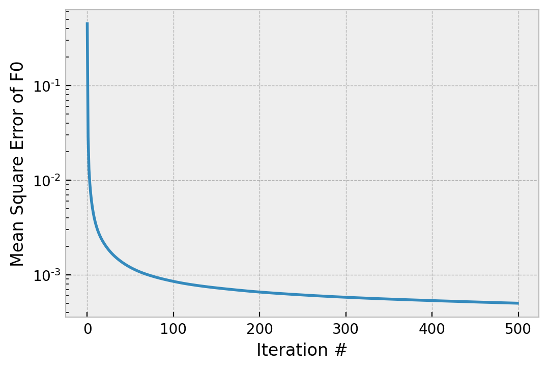
cost vs iteration for Misel’s two PSF algorithm

We can see two things: Misel’s algorithm converges with something like 1/x, and the data consistency bottoms out around 1e-3, similar to Gerchberg-Saxton. When we compare the phases, I will plot the absolute phase of each, since I think it will be a bit more clear:

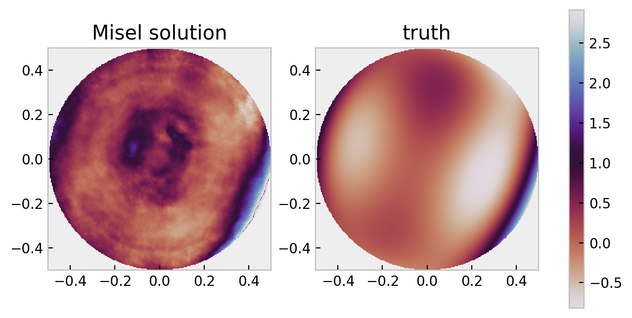
comparison of the phase found by Misel’s algorithm and

A small amount of extra code is needed to bring the complex field estimate at plane 0 back to a pupil plane, so we can compute the phase in the appropriate plane:

pupil = fft.fftshift(fft.ifft2(psf00))
ang = np.angle(pupil)
ang[absg<.1] = np.nan

In this plot, it looks like Misel’s algorithm didn’t work well at all, but if close attention is paid some of the “high frequency” features are very well found; the rapid phase ramps near the edges of the pupil. The very low frequencies are about right, too (if you squint, the astigmatic feature in roughly the 1 o’clock axis is well found). Perhaps troubling may be that there are some high frequency phase features that are ficticuous. However, recall that we can initialize an algorithm like GS or CG from a random phase (extremely high frequency features!) and it will converge to the smooth, low order solution.

“Serious” Use of Misel’s Algorithm

It is likely clear from the above results, however short, that using only Misel’s algorithm is not very great. The value of $3\lambda$ as the defocus parameter is a moderate number. When using phase diversity, the amount of diversity is a new parameter the phase retrieval user must choose well. Bruce Dean has a very nice paper on diversity selection, for those interested. As the defocus is made larger, Misel’s algorithm does worse and worse with high frequencies, and better and better with low frequencies.

One mistake that has been made a few times in the published literature is to claim that that Misel’s algorithm is strictly a two plane algorithm. While that is true exactly as prescribed, there is no reason one cannot transport between N planes and apply N amplitude constraints. There is a combinatorial problem of what order to move between the planes, but having to make a choice should not preclude implementation. It would be reasonable, for example, to move between the defocus planes in sequence, or to ping pong between defocus 1, focus, defocus 2, focus, […] defocus N, focus. Or middle out, going to nearer foci before further foci. Or outward in, from focus to further, and so on.

A “serious” implementation of focus diverse phase retrieval will essentially use a “recipe,” in which if Misel’s algorithm is used to implement the diversity, the whole algorithm will oscillate between using CG or GS iterations, and Misel iterations, which has some concept of greater convergence. This depends on each algorithm moving always in “the right” direction and never “the wrong” – things will never converge well if the two methods fight each other, or one undoes the other. The higher order recipe must be careful of this. If using CG, then one should be mindful to cool the algorithm, with a value of $h_k$ nearer to 0.5 than 1, during secondary or tertiary visits to the CG process, after blocks of Misel iterations.

Closing remarks on iterative transform focus diversity

One beautiful aspect of Misel’s algorithm is that it is structurally extremely similar to GS or CG, so experience with the latter two somewhat translates to Misel’s algorithm, and the similarity of implementation can make it easy to adapt the latter into the former. The multiple paths to implement multiple planes of focus diversity is somewhat a weakness. The curse of choice.

The use of angular spectrum in this instance to transport between planes produces much higher frequency (i.e., more aliasing prone) quadratic phases than other methods. For example, one could go from the “in focus” PSF back to the pupil, and apply a much smaller quadratic phase there than in the the angular spectrum domain.

Misel’s algorithm is similar to GS or CG in that it is an iterative transform method. It brings all the same weaknesses, for example susceptibility to phase wrapping and other errors, and need to fit the phase if you wish to extract polynomial coefficients. The latter is complicated by the need for registration and other problems, as well as crosstalk from out-of-band phase “modes” (noise, false diamond turning marks, etc).

What’s next?

At this point, we have walked through the majority of iterative transform phase retrieval, as it applies to image based wavefront sensing. A historical perspective is that this concludes a tour of the state of the art in the 1970s and 1980s, 40 to 50 years in the past. In the next posts, we will discuss the advancements of the new millennium. Notably, we will not discuss curvature wavefront sensing, developed by Roddier and Roddier, as well as Thurman independently. I acknowledge that these are also image based wavefront sensing methods, but I am not that knowledgeable on them and cannot give a good tutorial.