Phase Retrieval III: Making Conjugate Gradient Great

Introduction

In the last post I showed reference implementations of several common iterative transform Phase Retrieval algorithms. I alluded to Conjugate-Gradient being the most superior of them. In this post, we will do a very small amount of forward modeling and show how to make Conjugate Gradient even better than its most naïve version is. Before getting too far into that, I want to point out again that these are all iterative algorithms that “happen” to work. One is not always better than the other, although CG is usually superior to GS, and especially has more knobs to turn if it’s not working well.

Before we can tackle the reverse mode problem (PSF => phase) we need to do the forward mode problem (phase => PSF). For that, we’ll use the v0.20 development branch of prysm, my library for physical optics; you could use another if you prefer. Without further elaboration, we take up to 10 nm RMS each of Z3..Z16 Noll Zernike polynomials as the phase, and use a uniform circle for the amplitude of the pupil.

(editorial note, I intended to exclude all tilt but made a typo, the lower bound of 3 was meant to be 4. There is no loss of generality from the inclusion (or exclusion) of tilt. Large tilts are a problem for iterative transform phase retrieval, but the tilts here are small.)

import numpy as np

from scipy import fft

from prysm import coordinates, geometry, polynomials, propagation, wavelengths, fttools

import praise

from matplotlib import pyplot as plt
plt.style.use('bmh')


np.random.seed(20210425)

x, y = coordinates.make_xy_grid(256, diameter=2)
r, t = coordinates.cart_to_polar(x,y)
dx = x[0,1]-x[0,0]

nms = [polynomials.noll_to_nm(j) for j in range(3,16)]
coefs = np.random.rand(len(nms)) * 10  # [0, 10] nm rms
basis = list(polynomials.zernike_nm_sequence(nms, r, t))

phs = polynomials.sum_of_2d_modes(basis, coefs)
amp = geometry.circle(1, r)
wvl = wavelengths.HeNe

wf = propagation.Wavefront.from_amp_and_phase(amp, phs, wvl, dx)
psf = wf.focus(1, Q=2)
psf = abs(psf.data)**2

absg = fttools.pad2d(amp, Q=2)
phs_guess = np.zeros_like(absg)

The variable absg contains the transmission of the pupil, and phs_guess the initialization for the algorithm (zero phase error; colloquial for “no knowledge”).

We then do the reverse-mode problem for a fixed number of iterations (500):

with fft.set_workers(2):
    gsp = praise.GerchbergSaxton(psf, absg, phs_guess)
    erp = praise.ErrorReduction(psf, absg, phs_guess)
    sdp = praise.SteepestDescent(psf, absg, phs_guess, doublestep=False)
    cgp = praise.ConjugateGradient(psf, absg, phs_guess, hk=1)
    for i in range(500):
        gsp.step()
        erp.step()
        sdp.step()
        cgp.step()

As a reminder, Gerchberg-Saxton (GS) and Steepest Descent (SD) are the same when doublestep=True. The above results in the following Fourier (PSF) domain error metrics over time:

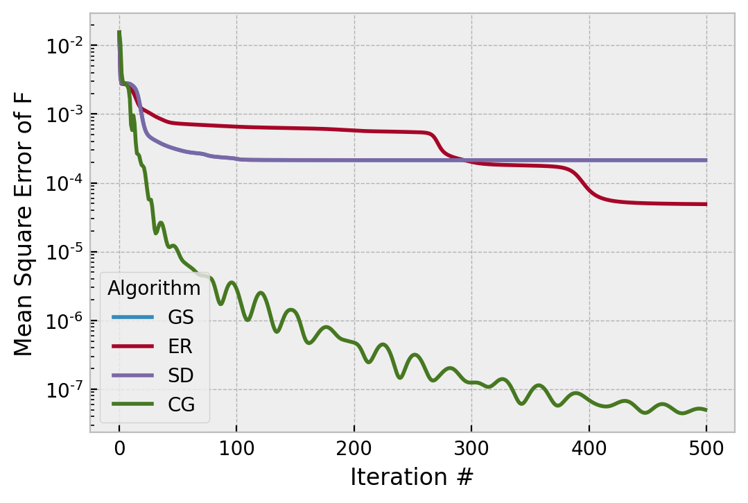
SD and GS follow indistinguishable trajectories, but in this particular example CG is doing a whopping 3 orders of magnitude better in the asymptote, and GS has fully stagnated. Since this error metric is computed in E field, in intensity (what is measured) it is 6 orders of magnitude better. That is quite extreme, but the oscillations in its trajectory imply something about its tuning is not optimal. We shouldn’t expect a deeper minimum, because 1e-7^2 is about 1e-14, not very far from double precision perfect. We can try pushing harder by using hk=1.5, to see if CG will go even faster:

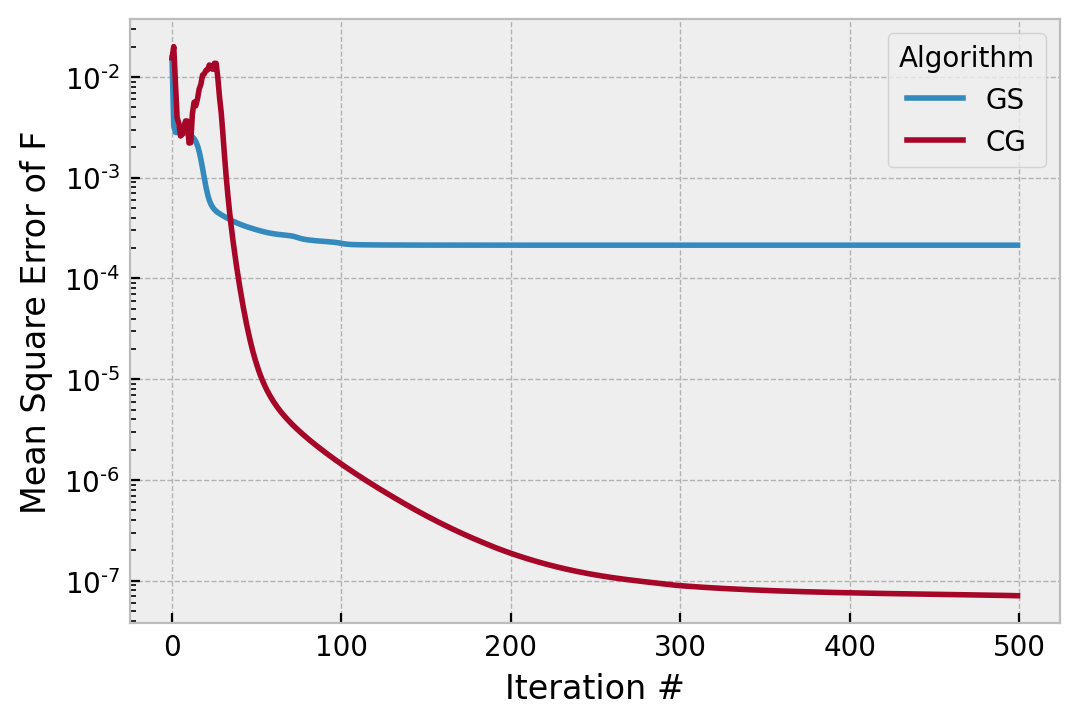
This didn’t make CG totally blow up, and its convergence is smooth everywhere. The initial divergence implies this is near a stability limit for this particular true phase and amplitude. It crosses 1e-6 (of no particular importance) around iteration 100, which is faster. Setting hk=2 for all iterations results in CG finding a solution 10x worse than if we had hk=1 for all iterations. If we slow it down with hk=0.5,

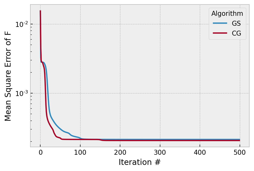
we can see it doesn’t really work any different to Gerchberg-Saxton.

Since we are primarily interested in making CG converge in a more or less monotonic way (you wouldn’t want to stop on the top of one of the ripples in the first image), we can simply slow it down by “cooling” hk over time:

gsp = praise.GerchbergSaxton(psf, absg, phs_guess)
cgp = praise.ConjugateGradient(psf, absg, phs_guess, hk=1)
for i in range(500):
    if i>0 and i % 100 == 0:
        cgp.hk *= 0.75
    gsp.step()
    cgp.step()

This is similar to the way the temperature of simulated annealing reduces over time, or changing from a driver to a putter in golf. The factor of 0.75 is another parameter to think about, and will result in a gain sequence of [1, .75, .5625, .421875] for this number of total iterations. We can see the effect is largely to smooth the convergence of CG, without perturbing its ultimate solution:

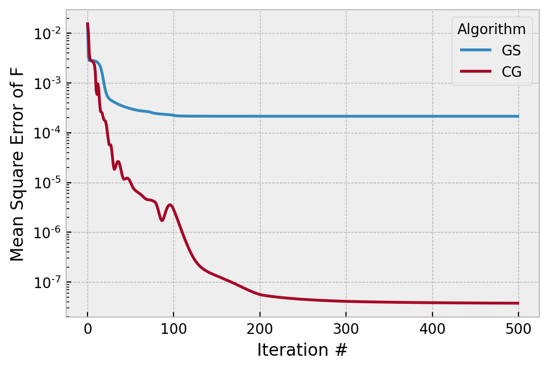
Note especially that it followed exactly the same path for iteration 0..100, and then converged both faster and more smoothly.

In this case, we could stop after 200 iterations.

But how good did they do, really?

The Fourier domain cost function used to monitor convergence of the algorithms is good insofar as it is a measure of the algorithm’s performance without use of external measurements. However, were there additional phases that produced the same PSF, this would be non-unique and we could be deceived by the error metric. In a simulation study, we can always compare the true phase to the retrieved phase, since both are known. We do so simply:

# minimum processing
padded = fttools.pad2d(wf.data, Q=2)
phs_true = np.angle(padded)

g_gs = praise.recenter(gsp.g)
g_cg = praise.recenter(cgp.g)
g_gs = np.angle(g_gs)
g_cg = np.angle(g_cg)
mask = absg < .9
g_gs[mask] = np.nan
g_cg[mask] = np.nan
phs_true[mask] = np.nan

g_gs -= np.nanmean(g_gs)
g_cg -= np.nanmean(g_cg)
# no need to do that to true, already zero mean

fig, axs = plt.subplots(figsize=(8,4), ncols=2)
axs[0].imshow(g_gs, clim=clim, extent=[-1,1,-1,1], cmap='twilight_r')
im = axs[1].imshow(g_gs-phs_true, clim=clim, extent=[-1,1,-1,1], cmap='twilight_r')
fig.colorbar(im, ax=axs)
axs[0].set_title('GS solution')
axs[1].set_title('GS solution - truth')
for ax in axs:
    ax.grid(False)
    ax.set(xlim=(-.5,.5), ylim=(-.5,.5))

The minor wall of matplotlib code produces this figure:

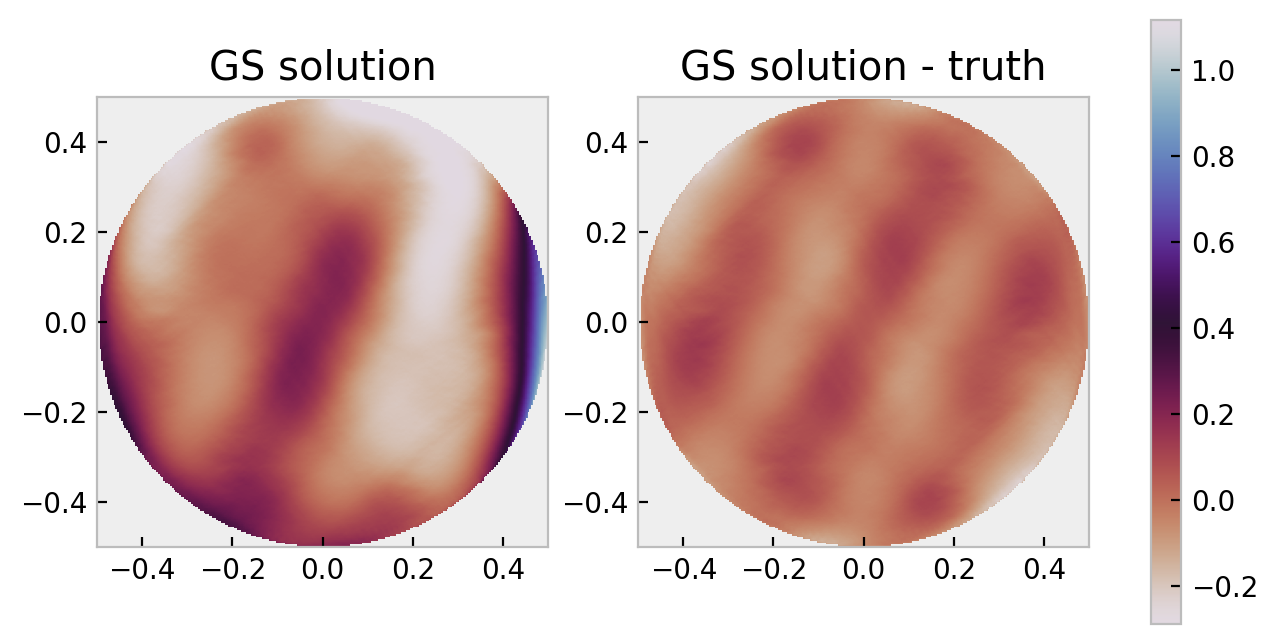
The colorbar scale is in radians. We can compute nicer statistics:

from prysm.util import rms, pv
rms(diff), pv(diff)

0.06412741333956434, 0.379369672400966

These compare to the same for phs_true of 0.184, 1.404, which is about a part in three fractional error. As a reminder, there are $2\pi$ rad per $\lambda$ of OPD, so 0.064 rad ~= $\lambda/100$.

The same comparison for CG reveals:

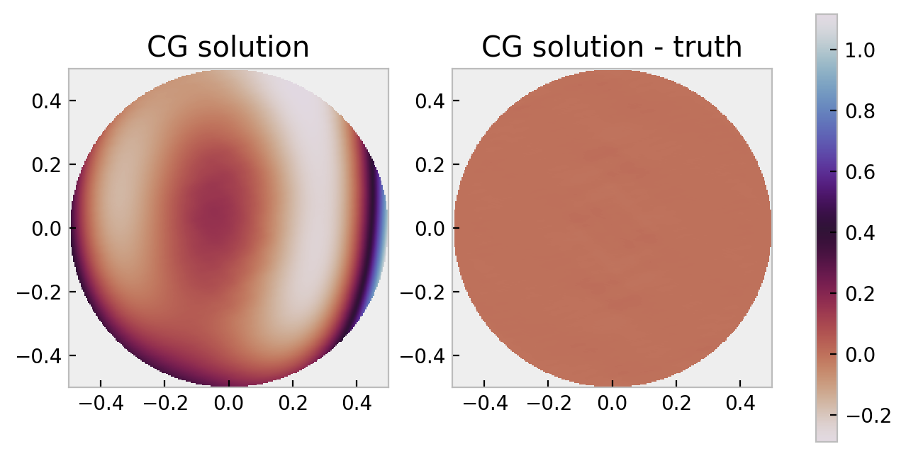
This has an RMS, PV difference of 0.00204, 0.01696 rad or ~= $\lambda/3000$ RMS. More impressive may be the $\lambda/400$ class PV accuracy.

Most of the error in the GS solution is higher frequencies (more cycles per aperture) which is an error source that can be reduced by inclusion of phase diversity.

If you would like to see CG really do fantastically better than GS, increase the scale factor on the coefficients from 10 to 50.

Thus far, it’s been seen that these algorithms work very well, and one may not wont for more. In the next post we will examine some of the dynamic range constraints of these algorithms, and how those constraints are addressed (diversity).