Introduction

Commercial interferometers are most often either Fizeau or Twynman-Green in their geometry. In order to measure the phase error in the test arm, the beam is divided and one half sent to a reference surface. The test and reference beams interfere at the camera, forming fringes which the elves in the instrument convert into a wavefront error map. You may also have built a michelson interferometer, which is broadly the same but has matched path lengths between the test and reference arms, enabling it to function with broad-band light.

What all of these have in common is the comparison of the test arm to a reference surface. The non-zero error in the reference surface places a lower bound on the accuracy of the instrument, even with calibration.

If you wish to measure wavefront errors of less than 1 nm RMS, the above varieties are driven to extremes in the fabrication of the reference surface and design of the instrument to limit internal errors such as retrace error.

In the world of extreme ultraviolet lithography, optics must be polished down to figure errors in the 50 pm RMS regime. The interferometers to make these measurements must be of 10 pm RMS class, and must operate at the operating wavelength near 13.5 nm. These challenges have motivated ASML, Zeiss, and their partners to develop an old idea to extreme levels of both accuracy and precision: the point diffraction interferometer, or PDI.

The concept of a PDI is that by placing a pinhole somewhere in an optical system on an otherwise semi-opaque substrate, a spherical wave will be generated which interferes with the remainder of the light in the far field. This spherical wave is completely unaberrated, and so the instrument has no errors due to a reference surface. That property is very desireable when extremely high accuracy is required. The geometry is generally showen in this figure:

Here I show the pinhole at the focus of a beam. This is the same geometry as a phase contrast wavefront sensor, except with a PCWFS instead of a pinhole there is a phase bump (or hole). The PDI was first invented in 1933, one year prior to Zernike’s discovery of phsae contrast. The original geometry called for the pinhole to be several $\lambda/D$ away from the core of the PSF. This geometry produces resting tilt fringes, with which deviation from straight lines can be evaluated by eye. However, by placing the pinhole in a region where the PSF is naturally dark, very little light is shone on it, and even less will pass through it. This makes the radiometric efficiency truly awful, and the substrate must have R ~= 0.001% for the test and reference arms to have equal power and the fringes to have good visibility. When the pinhole is placed in the focus as in my figure, the sign of the phase is ambiguous and there is no mechanism for resolving the ambiguity.

The exceptionally poor throughput of the more off-axis geometry, free of the sign ambiguity problem has made PDIs something of a novelty in the century since their invention. However, in the 90s some very brilliant people at Livermore discovered how with a diffraction grating, the efficiency could be improved by 40,000x, placing the PDI on equal footing to other types of interferometers, in terms of throughput.

The Medecki Interferometer

By placing a diffraction grating in the preceding pupil, multiple foci are created. And, if the beam is monochromatic they are all coherent to each other. A pinhole can be placed at one focus, and a simple window placed at the other on an otherwise opaque substrate. The two beams are coherent, one has had its aberration content destroyed, and their separation in the focal plane means there is a large phase tilt between them. This geometry is shown in the following figure:

The particulars of the focal plane mask depend on the particulars of the chosen grating. With either a square/binary or sine amplitude grating, order 0 is the brightest and receives the pinhole treatment. One of the +/- 1 orders is the next brightest, and gets a window placed at it. The window can be any shape.

Thinking only about the window for a moment, the focal plane is related to the pupil plane via a Fourier transform. By having a finite window, in effect we are low-pass filtering the beam. This is why the image in the figure has some subtle radial rings; the number of rulings is very low so that the tilt fringes are visible at low resolution, and consequently the window is only a few $\lambda/D$ in diameter, and the pupil is significantly low-pass filtered. In a practical implementation, there might be, say, 160 rulings per pupil diameter, several times more than are in the figure.

Because the resting image contains a large number of tilt fringes, single-shot interferometry is possible. However, single-shot interferometry is fraught with difficulties due to ambiguous parameters in experimental data (how many tilt fringes are there? Where is the edge/center of the aperture? etc…). Phase shifting is still highly desireable, and can be achieved by simply translating the grating in the axis orthogonal to its rulings. This has an added creature comfort that the grating rulings are likely 100s to 1000s of microns apart, and so a full $2\pi$ phase shft is 100s to 1000s of microns of motion, as opposed to just 100s of nm in, say, a Fizeau. This means the phase shifter accuracy requriements are significantly reduced.

Forward Modeling

The Phase Shifting Point Diffraction Interferometer (PS/PDI) or Medeki interferometer is practically begging to be modeled, when one is given a modeling package capable of modeling coronagraphs. Recall that I have been saying the pinhole is smaller than $\lambda/D$ in diameter. Then, to well-model a circle requires considerable oversampling, say Q=16. E.g., if the pupil fits in a 256x256 region, the total array FFT’d would be 4096 across. And, recall too that we need to model a sine or square wave with a hundred or two hundred cycles per aperture. So we really need >= 512x512 on the pupil. With contemporary FFTs this would be brutal and extremely slow; in the words of Raymond Hettinger, “there must be a better way.”

The world of coronagraphy has brought to us the matrix DFT, and the adjacent world of image-based wavefront sensing has brought us the Chirp Z Transform. These techniques allow the computation of the focal field in only a small region, which may or may not be shifted from the origin. Then, modeling a PS/PDI is reduced to two pairs of MFTs or pairs of CZTs; one forward-and-back for the pinhole, and one forward-and-back for the window. In other words, given a function of the general flavor,

def to_fpm_and_back(wf0, fpm, shift=None):
  focal0 = mft(wf, shift=shift)
  focal1 = focal0 * fpm
  wf1 = imft(focal1, shift=shift)

Then we can model the system as,

def pspdi_model(wf0, pinhole, window, window_transmissivity):
  ref_beam = to_fpm_and_back(wf0, pinhole, shift=None)
  test_beam = to_fpm_and_back(wf0, window, shift=the_grating_period)
  total_beam = ref_beam + test_beam

This is not only extremely elegant, but it is also highly performant, and the array sizes in the focal region are driven primarily by the desired accuracy in the grayscale or monochrome shading of the pinhole and circular mask.

Anyone who has read this blog before will find it completely unsurprising that there is now a PS/PDI model in prysm which does exactly this, available from the prysm.experimental.pdi package. There are a few hundred lines of parameter munging and code to draw the gratings (etc) involved, but the core of the implementation is this set of four MFTs/CZTs.

A very slick benefit to this flavor of model is that the test and reference beams are available right there in the code, and so the power in them can be computed to optimize the window transmissivity. This is not possible with an FFT-based model, which will just compute total_beam directly. Though, in an FFT-based model the total power inside the pinhole and inside the window can be computed from the array in the focal region. That will still miss the divergence out of the pinhole, which could be dealt with by simply turning off the window or vice versa. That just requires several enormous FFTs and a side of patience.

I think I’ll stick with the MFTs.

Here and in the rest of the post, we’ll use this snippet of python and prysm to model the PS/PDI:

import numpy as np

from prysm import (
    coordinates,
    geometry,
    propagation,
    polynomials
)
WF = propagation.Wavefront

from prysm.experimental.pdi import (
    PSPDI,
    degroot_formalism_psi,
    ZYGO_THIRTEEN_FRAME_SHIFTS,
    ZYGO_THIRTEEN_FRAME_SS,
    ZYGO_THIRTEEN_FRAME_CS,
    unwrap_phase,
    evaluate_test_ref_arm_matching
)

from matplotlib import pyplot as plt

efl = 10
lam = .633
epd = 2
Q = 1024/901

fno = efl/epd
flambd = fno*lam

x, y = coordinates.make_xy_grid(1024, diameter=Q*epd)
r, t = coordinates.cart_to_polar(x, y)
rmod = r/(epd/2)
dx = x[0,1] - x[0,0]

aperture = geometry.circle(epd/2, r)
phs = polynomials.zernike_nm(4,0, rmod, t, norm=False)*50 # units of nm
wf = WF.from_amp_and_phase(aperture, phs, lam, dx)

N=160
inter = PSPDI(x, y, efl, epd, lam,
    test_arm_offset=N,
    test_arm_fov=N/2,
    grating_rulings=N,
    test_arm_samples=512,
    test_arm_transmissivity=0.01,
    pinhole_diameter=0.25,
    grating_type='sin_amp')
pak = inter.forward_model(wf, 0, debug=True)
ratio, I1, I2 = evaluate_test_ref_arm_matching(pak)
print(ratio)
# >>> ratio = 0.93

The imports are as long as the code; sorry not sorry. Walking through this, the block with epd, yadda, sets up a circular aperture with some spherical aberration in it.

The block starting from N=160 sets up a PS/PDI whose grating is an amplitude sinusoid with 160 rulings per aperture diameter. The window is 160 $\lambda/D$ away, the pinhole is a quarter $\lambda/D$ in diameter, and we keep just 0.0001% of the light in the test arm (transmissivity is $t$, not $T$; amplitude, not power). The reason we throw out so much light in the test arm still is that while an amplitude sine grating sends most light into order 0, the pinhole is tiny. If the pinhole were 1 $\lambda/D$ in diameter, the test arm transmissivity could be increased to 0.15 while still having nearly ideally balanced arms.

Optimization of these parameters is not really inside the scope of this post, these are a working set to continue with.

To put the PS in PS/PDI, the model is able to phase shift by translating the grating. The phase shift parameter is expressed in the sense that phase shifting algorithms want; $2\pi$ is a full shift regardless of grating parameters. That is, if an algorithm wanted images at $(-\pi, -\pi/2, 0, \pi/2, \pi)$ you would run the model with $-\pi$ and so on.

The details of different phase shifting algorithms is also outside the scope of this post. I recommend Peter de Groot and Leslie Deck’s excellent papers for the interested reader. We’ll use Zygo’s 13-frame algorithm (the one every verifire uses) and de Groot’s formalism for the reconstruction of wrapped phase from the individual images,

shifts = ZYGO_THIRTEEN_FRAME_SHIFTS
frames = [inter.forward_model(wf, s) for s in shifts]

These all caps variables are constants from the PDI module. The API here will almost certainly change to be more ‘ergonomic.’ For now, constants prefixed by SCHWIDER_ are also available for the famous 5-frame Schwider-Harihan algorithm.

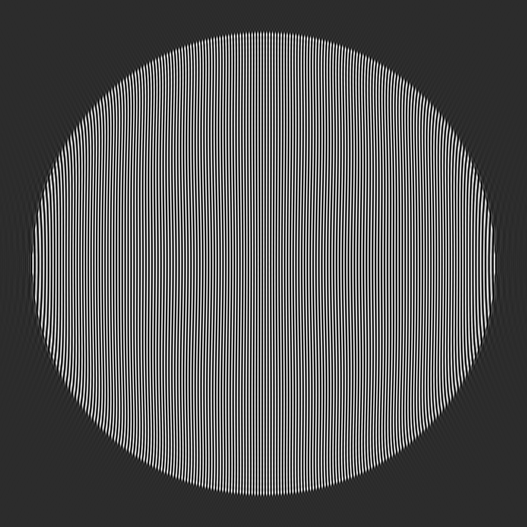
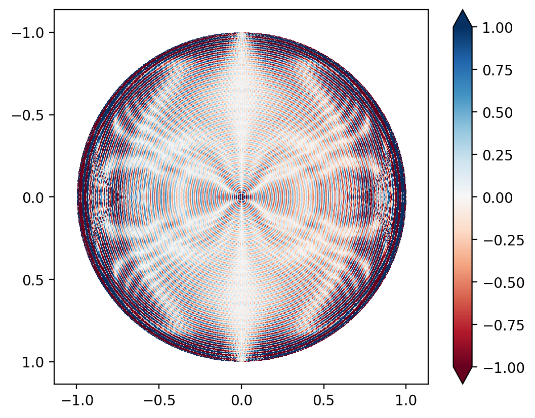
frames holds a list of synthetic (noiseless) images at each phase shift. An example with huge wavefront error can be downloaded at full resolution here. If you squint, you may be able to detect deviation from perfectly straight lines.

Reverse Modeling

The previous section ends with a bag of synthetic images in hand. To the limit of the model fidelity, if you built this system the camera would take those pictures. Now we need to turn a bunch of pictures of ever so slightly squiggly lines into a picture of a phase estimate. That process happens in a few steps:

1. Use the PSI algorithm to reconstruct the (wrapped) phase
2. Use a phase unwrapper to produce unwrapped phase
3. Do some post-processing, by way of piston/tip/tilt subtraction, masking, etc

We’ll do these one at a time. Step 1 is a one-liner:

ss, cs = ZYGO_THIRTEEN_FRAME_SS, ZYGO_THIRTEEN_FRAME_CS
reconstructed = degroot_formalism_psi(frames, ss, cs)

The wrapped phase is visualized in grayscale here. The eagle eyed might see the familiar “fish” shape of Coma. And that I swapped spherical for coma (sue me).

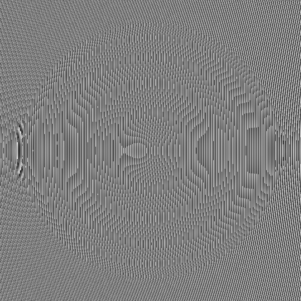
I have not, nor do I ever want to write a phase unwrapping code. The wonderful scikit-image has one of the most state-of-the-art algorithms included in the box, so prysm just wraps that. It is a notable point of sometihng that only works on CPU with prysm, which is rare these days. Anyway.

phs_fctr = (lam*1e3)/(2*np.pi)
recon2 = unwrap_phase(recon)
recon2.data *= phs_fctr

Here the phs_fctr converts radians to nanometers. The 1e3 is because we represent lambda with units of microns. The 2pi is because I assume the chief ray is normal to the focal plane. if it’s not, there should be an extra cosine obliquity in the denominator.

The contents of the array in recon2 is just going to look like a phase ramp, so we’ll use prysm’s interferometry module to go the rest of the way,

from prysm.interferogram import Interferogram

i = Interferogram(recon2.data.copy()*-1, recon2.dx)
i.mask(geometry.circle(epd/2, i.r))
i.remove_tiptilt()
i.remove_piston()
i.plot2d(interpolation='nearest', cmap='RdBu', clim=100)

After the processing, the picture looks like this:

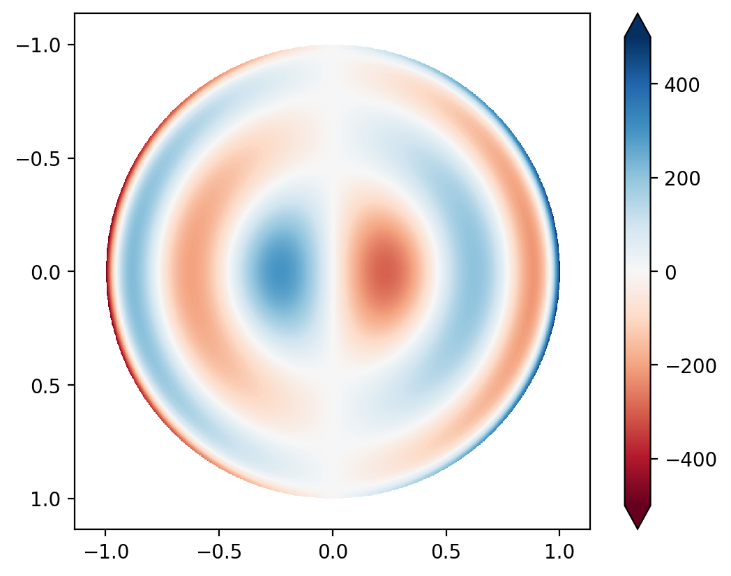
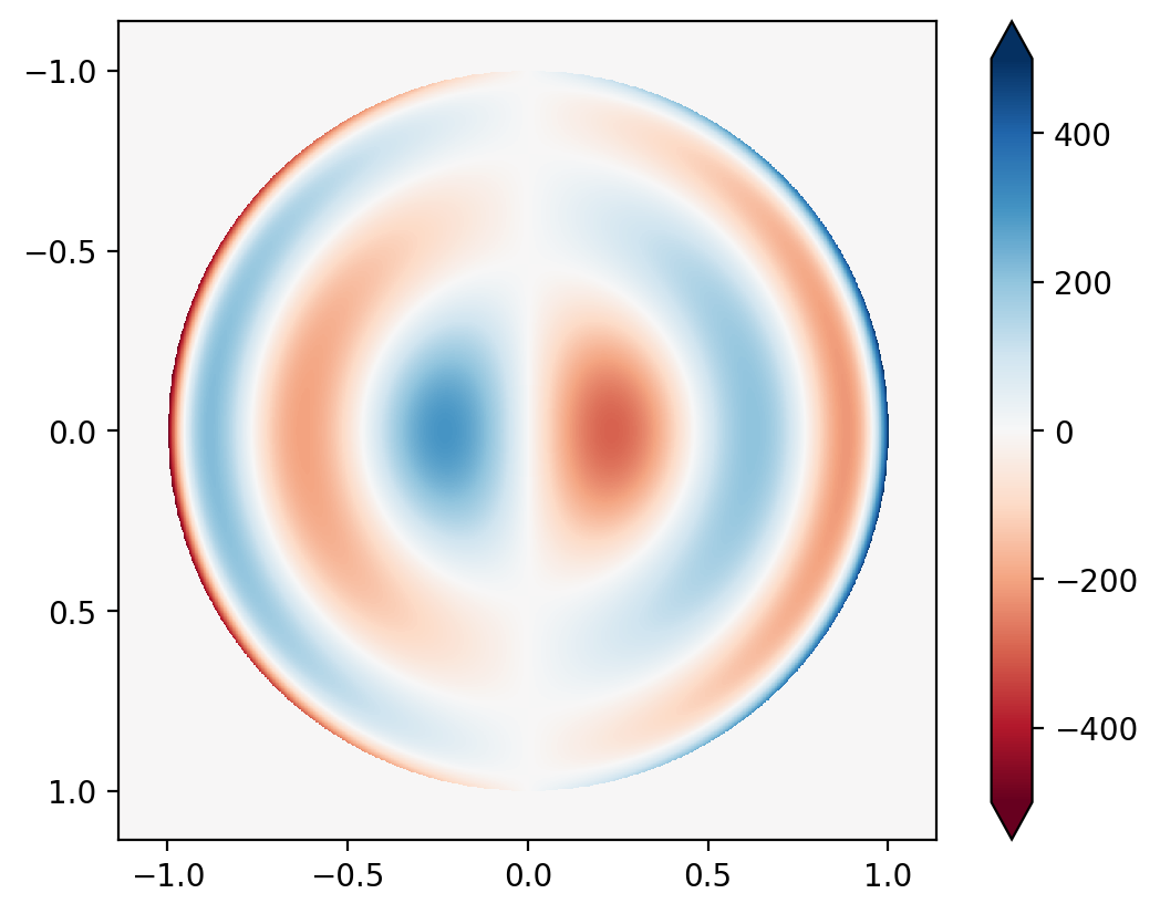
The answer we were expecting looks like,

And their elementwise difference looks like, (pay careful attention to the colorbar)

The RMS error is 2 nm, with a PV of 91.5 nm. Most of the error is concentrated at the very edge of the aperture, where the Gibbs ringing due to the band-limited nature of this interferometer topology makes things worse. Comparing the RMS of the error to the RMS of the expected value, it is less than 1%, i.e. the interferometer’s absolute accuracy, even on such a large wavefront error, is better than 99%.

Pretty cool technology. Those EUV people sure are smart.