Massively Faster Modeling of Segmented Telescopes
This post will discuss techniques that can be used to very quickly model segmented optical systems. Segmented systems have apertures or other surfaces which are made of several pieces, which are discontiguous. They look like:
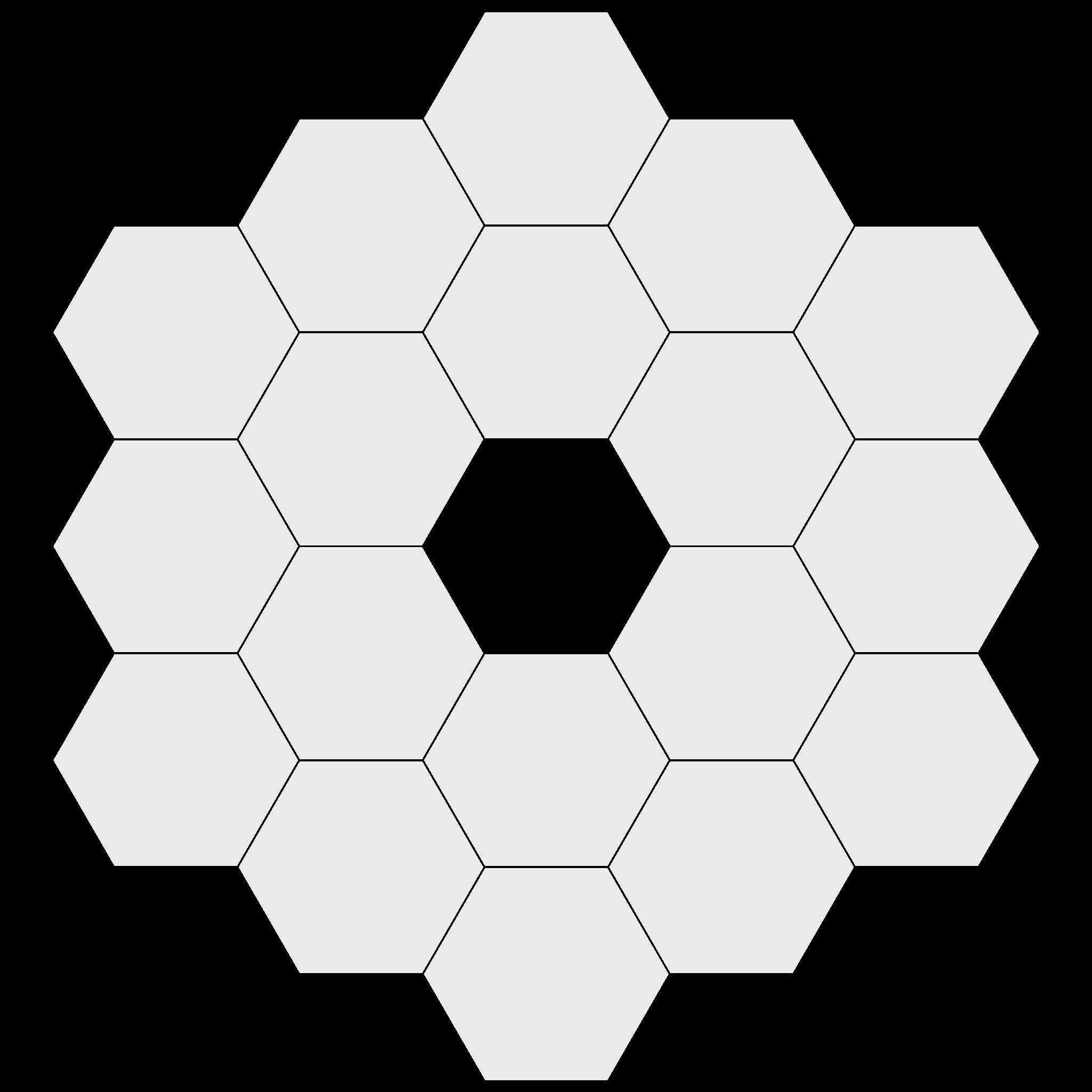 a JWST-like aperture without strut obscurations
Segmented systems introduce an interesting fork in the road of modeling. In a monolithic system, you can discuss the aberrations of the pupil for a given field angle, but in segmented systems you can talk about per-segment errors as well as errors that span the entire pupil. There exist some prior art in open source tools for modeling these. I will briefly highlight POPPY, the physical optics library produced by the Space Telescope Science Institute and collaborators. (Of course, many closed source programs exist, too.)
Presupposing that you wanted to produce a similar image, you would enter:
from astropy import units as u

from poppy import MultiHexagonAperture, Wavefront

w = Wavefront(npix=2048, diam=6.8*u.m)
h = MultiHexagonAperture(flattoflat=1.32, gap=0.007, rings=2);
h.get_transmission(w)
This is not the code I used to produce the image, and runs in 2.37 seconds. While such a timing is not completely unweildly – you could execute this many times per in a single workday, say – it does preclude the use of h.get_transmission in any performance sensitive code. A similar invocation with 16 rings for an EELT-like aperture would take a few minutes to run over the same array size, which is not really large enough for the number of segments in the EELT pupil (read as: this would get exponentially slower).
The algorithm within poppy is actually fairly complicated and weighs in at about 200 lines of code. One of its properties is that its execution time is linear in the number of segments:
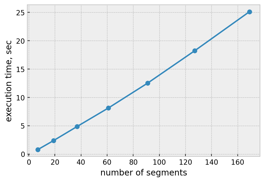 POPPY time taken to shade segmented hexagonal aperture vs segment count
Linear scaling quickly becomes limiting when you bang it against 10x or more increases in system parameters, as is the case with EELT’s 700+ segments vs JWST’s 18. EELT is exceptional, but LUVOIR-A has more than 100 segments, too.
A better algorithm adapts concepts from video game programming to perform computations on hexagonal grids. For background (and where I have taken these concepts), see Red Blob Games’ site. First we need just a few pieces of machinery for operating on a coordinate system with three bases in 2D:
from collections import namedtuple

Hex = namedtuple('Hex', ['q', 'r', 's'])


def add_hex(h1, h2):
    """Add two hex coordinates together."""
    q = h1.q + h2.q
    r = h1.r + h2.r
    s = h1.s + h2.s
    return Hex(q, r, s)


hex_dirs = [
    Hex(1, 0, -1), Hex(1, -1, 0), Hex(0, -1, 1),
    Hex(-1, 0, 1), Hex(-1, 1, 0), Hex(0, 1, -1)
]

def hex_dir(i):
    """Hex direction associated with a given integer, wrapped at 6."""
    return hex_dirs[i % 6]  # wrap dirs at 6 (there are only 6)

def hex_neighbor(h, direction):
    """Neighboring hex in a given direction."""
    return add_hex(h, hex_dir(direction))


def hex_to_xy(h, radius, rot=90):
    """Convert hexagon coordinate to (x,y), if all hexagons have a given radius and rotation."""
    if rot == 90:
        x = 3/2 * h.q
        y = np.sqrt(3)/2 * h.q + np.sqrt(3) * h.r
    else:
        x = np.sqrt(3) * h.q + np.sqrt(3)/2 * h.r
        y = 3/2 * h.r
    return x*radius, y*radius


def scale_hex(h, k):
    """Scale a hex coordinate by some constant factor."""
    return Hex(h.q * k, h.r * k, h.s * k)
In (overly) brief, this machinery allows us to operate on hex ‘tiles’ with coordinates $(q, r, s)$ and has a reverse transformation back to $(x,y)$ given the radius (half vertex-to-vertex) of each hexagon.
Given this machinery, we can very succinctly find all hexagons in a ring:
def hex_ring(radius):
    """Compute all hex coordinates in a given ring."""
    start = Hex(-radius, radius, 0)
    tile = start
    results = []
    # there are 6*r hexes per ring (the i)
    # the j ensures that we reset the direction we travel every time we reach a
    # 'corner' of the ring.
    for i in range(6):
        for j in range(radius):
            results.append(tile)
            tile = hex_neighbor(tile, i)

    # rotate so that the first element is 'north'
    for _ in range(radius):
        results.append(results.pop(0))

    return results
Then use this to shade an onion of rings:
def composite_hexagonal_aperture(rings, segment_diameter, segment_separation, x, y, segment_angle=90):
    if segment_angle not in {0, 90}:
        raise ValueError('can only synthesize composite apertures with hexagons along a cartesian axis')

    flat_to_flat_to_vertex_vertex = 2 / truenp.sqrt(3)
    segment_vtov = segment_diameter * flat_to_flat_to_vertex_vertex
    rseg = segment_vtov / 2
    mask = regular_polygon(6, rseg, x, y, center=(0, 0), rotation=segment_angle)

    all_centers = [(0, 0)]
    for i in range(1, rings+1):
        hexes = hex_ring(i)
        centers = [hex_to_xy(h, rseg+segment_separation, rot=segment_angle) for h in hexes]
        all_centers += centers
        for center in centers:
            lcl_mask = regular_polygon(6, rseg, x, y, center=center, rotation=segment_angle)
            mask |= lcl_mask

    return mask
This algorithm is already faster than POPPY, taking 15.1 seconds to shade 7 rings. However, there is huge waste because we know a priori that most samples of the grid are irrelevant to any given hexagon. If we modify the inner loop a bit, we can only shade the hexagons on areas just larger than their support:
def _local_window(cy, cx, center, dx, samples_per_seg):
    offset_x = cx + int(center[0]/dx) - samples_per_seg
    offset_y = cy + int(center[1]/dx) - samples_per_seg

    upper_x = offset_x + (2*samples_per_seg)
    upper_y = offset_y + (2*samples_per_seg)

    # clamp the offsets
    if offset_x < 0:
        offset_x = 0
    if offset_x > x.shape[1]:
        offset_x = x.shape[1]
    if offset_y < 0:
        offset_y = 0
    if offset_y > y.shape[0]:
        offset_y = y.shape[0]
    if upper_x < 0:
        upper_x = 0
    if upper_x > x.shape[1]:
        upper_x = x.shape[1]
    if upper_y < 0:
        upper_y = 0
    if upper_y > y.shape[0]:
        upper_y = y.shape[0]

    return slice(offset_y, upper_y), slice(offset_x, upper_x)


def composite_hexagonal_aperture2(rings, segment_diameter, segment_separation, x, y, segment_angle=90, exclude=(0,)):
    if segment_angle not in {0, 90}:
        raise ValueError('can only synthesize composite apertures with hexagons along a cartesian axis')

    flat_to_flat_to_vertex_vertex = 2 / truenp.sqrt(3)
    segment_vtov = segment_diameter * flat_to_flat_to_vertex_vertex
    rseg = segment_vtov / 2

    # center segment
    dx = x[0,1] - x[0,0]
    samples_per_seg = rseg / dx
    # add 1, must avoid error in the case that non-center segments
    # fall on a different subpixel and have different rounding
    # use rseg since it is what we are directly interested in
    samples_per_seg = int(samples_per_seg+1)

    # compute the center segment over the entire x, y array
    # so that mask covers the entirety of the x/y extent
    # this may look out of place/unused, but the window is used when creating
    # the 'windows' list
    cx = int(np.ceil(x.shape[1]/2))
    cy = int(np.ceil(y.shape[0]/2))
    offset_x = cx - samples_per_seg
    offset_y = cy - samples_per_seg

    upper_x = offset_x + (2*samples_per_seg)
    upper_y = offset_y + (2*samples_per_seg)
    center_segment_window = (slice(offset_y, upper_y), slice(offset_x, upper_x))

    mask = np.zeros(x.shape, dtype=np.bool)
    if 0 in exclude:
        mask = np.logical_xor(mask, mask)

    all_centers = [(0, 0)]
    segment_id = 0
    segment_ids = [segment_id]
    windows = [center_segment_window]
    xx = x[center_segment_window]
    yy = y[center_segment_window]
    local_coords = [
        (xx, yy)
    ]
    center_mask = regular_polygon(6, rseg, xx, yy, center=(0, 0), rotation=segment_angle)
    local_masks = [center_mask]
    for i in range(1, rings+1):
        hexes = hex_ring(i)
        centers = [hex_to_xy(h, rseg+segment_separation, rot=segment_angle) for h in hexes]
        all_centers += centers
        for center in centers:
            segment_id += 1
            segment_ids.append(segment_id)

            local_window, _ = _local_window(cy, cx, center, dx, samples_per_seg)
            windows.append(local_window)

            xx = x[local_window]
            yy = y[local_window]

            local_coords.append((xx-center[0], yy-center[1]))

            local_mask = regular_polygon(6, rseg, xx, yy, center=center, rotation=segment_angle)
            local_masks.append(local_mask)
            if segment_id in exclude:
                continue
            mask[local_window] |= local_mask

    return segment_vtov, all_centers, windows, local_coords, local_masks, segment_ids, mask
This version of the code has a new assumption that the array was (FFT-)centered on zero, but that’s just fine for its application. It seems much larger, but the bulk of that has to do with all the extra stuff it returns at the same time. When we benchmark this, we find that it has very weak dependence on the number of hexes in the array:
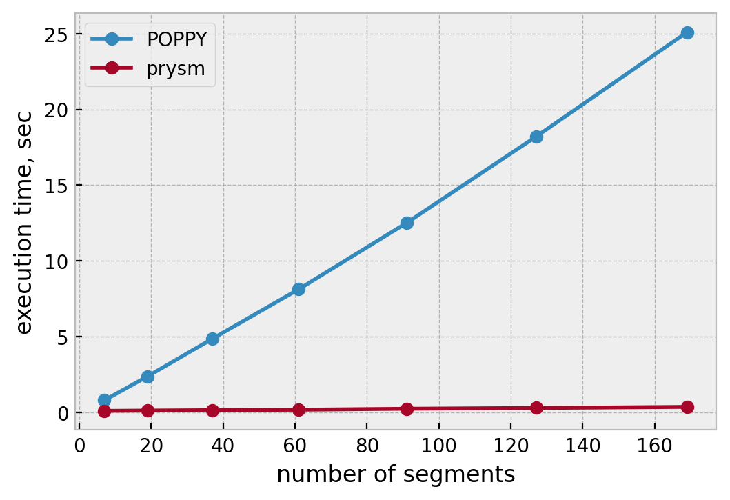 POPPY vs prysm v0.20 alpha time taken to shade segmented hexagonal aperture vs segment count
When you project this out to an EELT-like aperture, the performance gain is about 200x. For those curious, the tabular data on the timings looks like:
| # rings | # segs | POPPY | prysm |
|---|---|---|---|
| 1 | 7 | 0.79 | 0.091 |
| 2 | 1 | 2.37 | 0.114 |
| 3 | 37 | 4.85 | 0.141 |
| 4 | 61 | 8.12 | 0.170 |
| 5 | 91 | 12.5 | 0.235 |
| 6 | 127 | 18.2 | 0.287 |
| 7 | 169 | 25.1 | 0.359 |
Essentially, this algorithm only considers each pixel (approximately) once. The other things returned are useful information. For example, we can identify the segments by unique IDs and visualize that information:
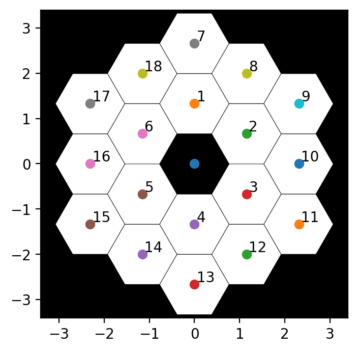
The exclude keyword argument can also be used to remove some segments. This makes it fairly trivial to handle any segment-quantized obscurations (like LUVOIR-A missing an inner ring), or simulate the effect of missing segments and other interesting questions (say, excluding the majority of segments for some metrology application). The returns, in order, are:
- the segment vertex-to-vertex distance, needed to normalize any local coordinates
- the center coordinates of each segment
- the windows (slice objects) into the main array that just enclose each segment
- the local coordinates (x, y) of each segment
- the local mask for each segment, needed to composite anything on a per-segment basis
- the ID for each segment
- the composited mask
This allows more efficient code. Truly efficient code is a bit more elaborate, so I will show a relatively inefficient algorithm here. But if you wanted to inject random tip/tilt into the segments you could do, for example:
def random_segment_tilt(stdev, indices, local_coords, local_masks, segment_ids, exclusions, segment_radius, buffer=None, shape=None):
    # this is just an example, the modes should be cached on a per-segment basis and not computed inline
    stdev = stdev / np.sqrt(2)  # for x, y components
    xvals = np.random.normal(0, stdev, size=len(indices))
    yvals = np.random.normal(0, stdev, size=len(indices))
    if buffer is None:
        buffer = np.zeros(shape, dtype=np.bool)

    for slices, (x, y), lcl_mask, id_, mx, my, in zip(indices, local_coords, local_masks, segment_ids, xvals, yvals):
        if id_ in exclusions:
            continue

        r, t = cart_to_polar(x,y)
        r/= segment_radius

        tx = zernike_nm(1, 1, r, t)
        ty = zernike_nm(1, -1, r, t)
        local_tilt = tx * mx + ty * my
        local_tilt[~lcl_mask]=0
        buffer[slices] += local_tilt

    return buffer
The computation of the tilts, and adjustments of the coordinate grids inline can be removed and a lookup table of segment id => modes can be pre-computed, moving almost all the work out of any loops. Visually, this looks something like:
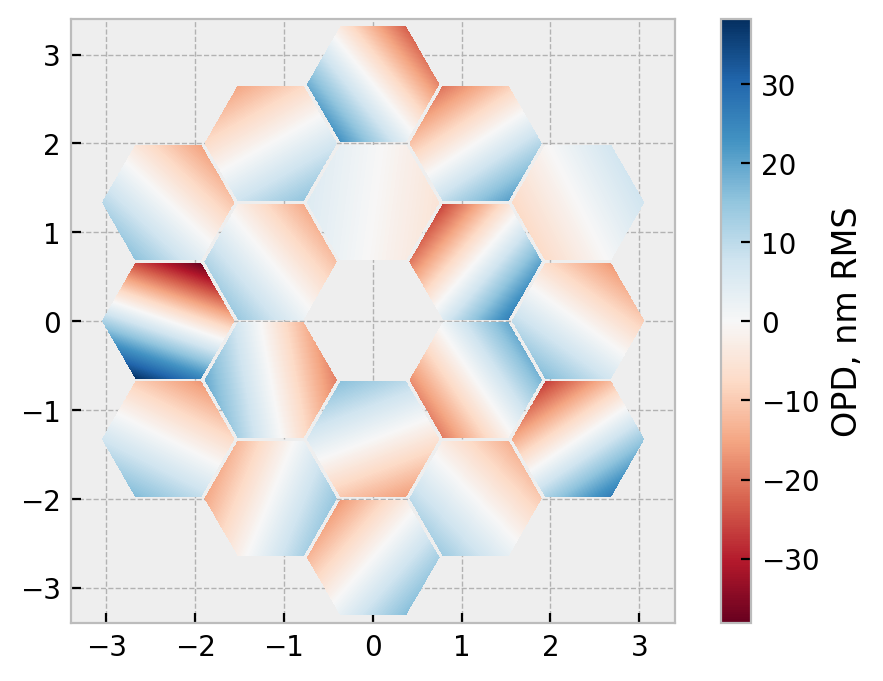 JWST-like aperture with random per-segment tilts.
This sort of modeling is useful to see, for example, how the multiple segments will form distinct, mutually coherent PSFs if the tilt is too large (this is a major metrology challenge in deploying James Webb):
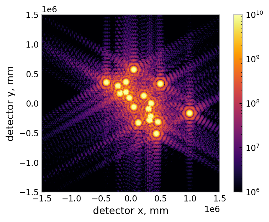 cluster of PSFs formed by a JWST-like aperture with per-segment tilts
Note that the tilts for this image-plane image are much larger than those shown above.
The code developed during the writing this post is located in the segmented submodule of prysm, currently quarantined to the v020 dev branch.
In Summary
To wrap this up, the use of hexagonal coordinates inspired by video game code to compute hex tile grids allows us to write elegant code to shade segmented apertures.
That code can be tweaked to remove computation over regions we know each segment does not exist in, improving performance by about two orders of magnitude for real systems that people want to analyze.
Exporting additional data products during the shading of the pupil, including several on a per-segment basis, allows one to write relatively elegant and fast code to model per-segment wavefront errors.
In aggregate, this can advance the state of the art in modeling segmented systems with physical optics by improving performance to such a degree that studies that were computationally infeasible can now be done.